1 Objective¶

This work is motivated as a verification exercise for the wavefront curvature sensing implementation on the Rubin Auxiliary Telescope. Achieving collimation on that telscope uses three effective degrees of freedom: 1) the z-position of the secondary, and 2) the combination of secondary tilt and x,y position. The latter two are degenerate over the modeset field of view of the Aux Tel system. Note that primary-to-secondary and secondary-to-focal plane spacing are linked and are not independently adjustable. Changing that ratio requires moving either the primary mirror positioning setpoint or the standoff distanace of the instrument from the Nasmyth flange.

Proper collimation places the optical axes of the primary and secondary mirrors line on a single line. Small positioning offsets can be compensated by introducing a tilt of the secondary. When the system is properly collimated, in an out-of-focus donut image the obscuration of the secondary mirror is centered on the primary pupil. Also, the surface brightness of the light is uniform. If the secodary is displaced, then the obscuration moves off center and a planar tilt in surface brightness appears.

Sequences of images were acquired with the secondary mirror displaced on an x-y grid. The resulting images were analyzed to ascertain the offset between the centers of the primary and secondary mirrors. In addition, a planar fit to the annular surface brightness was performed. The centroid offsets in x and y and the surface brightness gradient were fitted to the x,y mirror displacement in order to determine the best-position of the secondary. That can then be compared to the best-position as determined by the wavefront curvature code.

The secondary support spiders obscure the annular donut, and the images contain some cosmic rays and detector artifacts. This requires trimming pixel arrays to retain only meaningful surface brightness measurements.

2 Data¶

We used the data from the November 2021 run of AuxTel. specifically we used images seq_num 501-554 for this analysis. We found that our analysis was improved by driving the secondary further out of focus than the amount typically used for the wavefront curvature sensing. For the images analyzed here, the axial offset of the seecondary was 8 mm. The grid of latteral offsets spanned \(\pm\) 4 mm.

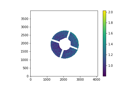
Figure 1 The initial cutout of a donut, before it has been normalized or gaussianized. the example used is sequence 502.

We first smooth out the image by running it through cv2.GaussianBlur(). This amounts to a low pass spatial filter that improves the signal to noise ratio. Next we normalize the flux across the donut. This is done by determining the normValue for the donut and a background skyValue the normalized image is then:

# We normalize and remove background sky values:
normValue = np.percentile(cutoutSmoothed, normPercent)
skyValue = np.percentile(cutoutSmoothed, skyPercent)

normImage = (smoothedImage - skyValue)/normValue

The normPercent and skyPercent are dependent on the date the data was taken and the brightness of the star that was imaged. For the analysis done of the donuts from the November 2021 run, we used ``normPercent``=90 and ``skyPercent``=15.

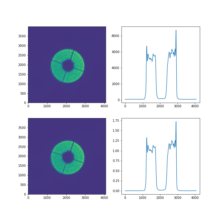
Figure 2 Top figures are the Gaussianized but not normalized donut, and a cross-section. The bottom two figures are the normalized versions of these. Same sequence used as above.

Next we use the normImage for determining a mask that will pick out only the useful donut part of the image. We convert this mask into a uint8 copy of the image, this last part is for finding finding the inner and outer cirlces only. While the mask is used both for this and for the gradient fit, see below.

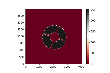
Figure 3 the mask obtained from the normImage using a maxclip value to cut out the mask, for the November 2021 run we used ``maxclip``=0.8.

For obtaining the circles we use the cv2.HoughCircles() to get the circle centers and radii. The parameters of the function are sequentially chosen to pick out the inner and outer edges of the annulus, respectively.

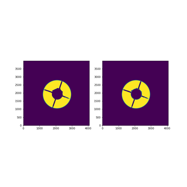
Figure 4 Left is just the outer-circle fitted, while right image is both circles added in.

3 Analyses¶

We analyzed the donut images using 2 different methods.

Our first method was to estimate the inner and outer rings of the donut, and their centers. If the image was perfectly in collimation we would expect their center’s to overlap. Since there are intentionally introduced secodary offsets we obtain a lists of centroid offsets dx and dy as a function of the secondary mirror postion. These offsets should be related to the position of the secondary mirror or Hexapod positions. we expect the relation to be described by

\[\begin{split}dx &= c_1 x_{hex} + c_2 y_{hex} + x_0\\ dy &= c_3 x_{hex} + c_4 y_{hex} + y_0\end{split}\]

Hence we can do a fit and obtain the matrix C and the offset \(\vec{O}\) from these we can then solve for the case that dx and dy = 0:

\[\vec{r}_\text{focus} = {\bf C}^{-1} (-\vec{O})\]

This is the centroid-based best-position of the secondary mirror, which can be compared to the values produced by the wavefront curvature code.

The second method is to instead look at the flux accross our donut. The flux is uneven because of the donut being out of collimation so we can fit the flux level accross the donut with a plane:

\[F = \Delta_x x_ + \Delta_y y + f_0\]

In turn we can then find a similar relation between the \(\vec{\Delta}\) and the Hexapod postions as we could with our first method. Finally solving for when the gradient of the plane is zero produces a separate estimate of the best-secondary-position.

3.1 Code-base¶

The code for used for the analysis is available in Stubbs laboratory groups github repo PCWG-Auxtel An example notebook of how to use the code is available in the technotes github repo.

4 Results¶

The results for this analysis is 2 estimates for the optimal secondary position. We can compare these to the reported secondary postion from the WaveFront sensor which was found to be (-3.85, 2.26)mm for the night in question. From our centroid and gradient analyses we obtain (-3.70,2.35)mm and (-3.93, 2.23)mm respectively. So we have that the focus reported by WFS lies between the collimation values that we found, but very close. Hence we feel this shows that the WFS is indeed working as intended.

Figure 5 The result of the second method vs. the WFS result. the arrows are the estimated gradient of the flux, indicated by direction and size, for each of the images used in the analysis.

Note

This technote is not yet published.

We built a module that can analyze donut images taken from the AuxTel to verify the focus estimation obtained from the wavefront estimator